MOHR Application Note:
TDR for Microwave/RF and Digital CablesTime-Domain Reflectometry (TDR)
TDR is a specialized form of closed-circuit radar developed for characterizing transmission lines, and is particularly useful for testing coaxial and twisted-pair cables and connectors found in modern microwave/RF and digital communications systems. A TDR can be thought of as a combination of a pulse generator and an oscilloscope, as shown in Figure 1. The pulse generator injects a transient wideband test signal into a transmission line, and the oscilloscope records the resultant reflections caused by impedance variations along its length. In practice, TDRs are usually specialized instruments because the oscilloscope and pulse generator must be closely linked in order to make accurate measurements. TDR is a "time-domain" method because, although TDR depends on wideband microwave/RF circuitry, measurements are made and usually displayed as a function of time rather than of frequency.
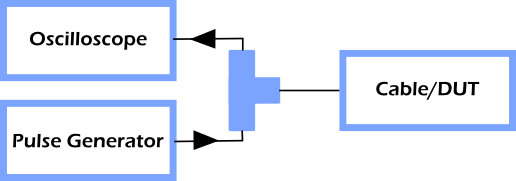
Figure 1: Diagram of a TDR. A TDR is essentially a special-purpose oscilloscope mated to a pulse generator. Multiple pulse-echo periods are usually used to build up a TDR waveform.
TDR Measurement Fundamentals
Vertical Measurements: Reflection Coefficient and Impedance
TDRs measure reflection coefficient, Γ(t), which is the ratio of the reflected to incident voltage at time t. The value of Γ ranges from -1 to +1, and is usually expressed in units of millirho, or 0.001·Γ. The reflection coefficient is dependent on the local impedance, ZL, and source impedance, Z0, according to the following relationship:
A perfect impedance match results in Γ=0, and an open and short result in G=+1 and -1, respectively. The measured reflection coefficient, Γ, can be used to estimate local impedance:
TDRs frequently have a fixed source impedance, usually 50 Ohms. Because of the non-linear relationship of measured reflection coefficient to calculated impedance, this is important when considering the accuracy of TDR impedance calculations. Figure 2 relates reflection coefficient to local impedance (Z_L) for a TDR with a fixed 50 Ohm source impedance.
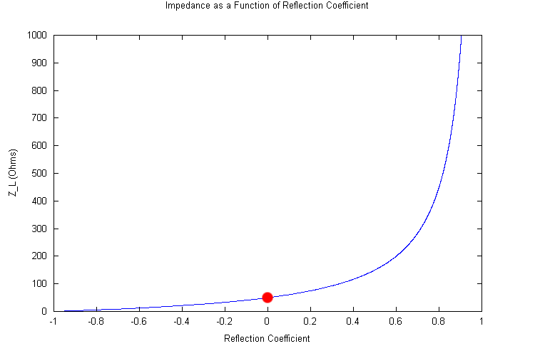
Figure 2: Relationship of calculated impedance to measured reflection coefficient for a 50 Ohm TDR system. Reflection coefficient range extends from short (-1) to open (+1). Red circle is at Γ=0 (50 Ohms). Due to the nonlinear relationship between reflection coefficient and impedance, for a given uncertainty in the measured reflection coefficient, the uncertainty in calculated impedance is increasingly large for increasing impedance values.
Accurate impedance estimates are relatively simple around the 50 Ohm source impedance, but become increasingly difficult above 200 Ohms, above which point minor uncertainty in reflection coefficient results in increasingly large uncertainty in calculated impedance. At 1,000 Ohms, for instance, accurate impedance estimates require extremely accurate, precise, and stable reflection coefficient measurements. Although a number of systems rely on high-impedance transmission lines, most TDR manufacturers do not specify accuracy above 200 Ohms. In contrast, the CT100 and CT100HF have been specifically designed to provide accurate impedance estimation from short-circuit to more than 1,000 Ohms over the 0-50°C operating range of the instrument.
Vertical Measurements: Return Loss and VSWR, FFT
TDR return loss is a lumped-parameter, logarithmic expression of the reflection coefficient:
where VI and VR are the incident and reflected voltages, respectively. A large return loss indicates that little signal is being reflected, consistent with a good source-load impedance match. Return loss can also be expressed as a negative number, depending on convention.
Voltage Standing-Wave Ratio (VSWR) is another way of expressing the reflection coefficient:
With a perfect match, VSWR=1. Increasing mismatch results in increasing VSWR, with values approaching infinity for open and short. Figure 3 depicts the open end of a 14.3 ft. coaxial cable with expected reflection coefficient, impedance, and VSWR measurements.
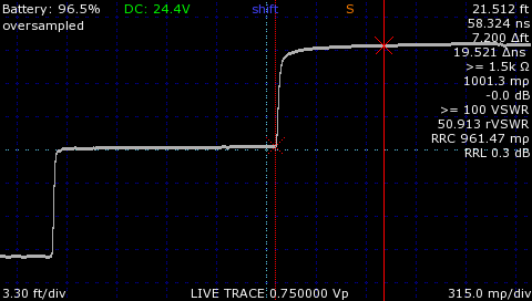
Figure 3: Open end of 14.3 ft. RG-58 coaxial cable. The right-hand cursor has been selected and there are expected reflection coefficient, impedance and VSWR measurements for an open fault. Relative measurements between the two cursors are also displayed.
S-parameter analysis is a well-developed technique using the Fast Fourier Transform (FFT) for linear decomposition of a TDR waveform into its constituent frequencies. Associated measurements include frequency-specific return loss and estimated cable insertion loss. A variety of calibration methods exist to reference TDR-based frequency-domain measurements to known standards so that accuracy at the test plane may be established. Further details of TDR frequency-domain analysis are presented elsewhere.
Horizontal Measurements: Velocity of Propagation (vp, VoP)
TDR horizontal measurements are fundamentally based on measurement of time rather than distance. Distance is calculated with the help of the known or estimated velocity of the test signal in the cable or device-under-test (DUT). The velocity of an electromagnetic signal along a transmission line, vp (or VoP), is related to the speed of light, c, and relative permittivity of the transmission line dielectric, εr, by the following relation:
The value of vp can be determined by testing a known length of cable or by referring to a manufacturer's specification. The better the accuracy of vp, the more accurate any associated distance or length measurements will be. Because TDR operators may not always appreciate the importance of using an accurate vp, uncertainty in vp is usually the single largest source of error in a TDR distance measurement. Likewise, using an accurate but imprecise vp also limits distance accuracy — a two-digit vp value provides a minimum distance uncertainty of 1%. This may not sound significant unless you consider the result in longer cables; for instance, a 1% uncertainty is equivalent to 10 m. in a 1 km cable.
If an accurate measurement is desired, it is usually worthwhile to carefully measure vp for the particular type of cable being tested. Measured vp may vary somewhat even for a given type of cable from production lot to production lot, so when in doubt, remeasure vp. CT100 Series TDRs allow the operator to specify vp to 6 digits to minimize error due to uncertainty in vp.
Horizontal Measurements: Distance-to-Fault and Length Measurements
Distance-to-Fault (DTF) and cable length are determined using the following relationship between distance, D, and time, t, accounting for the round-trip propagation of a TDR measurement:
Again, the major uncertainty in the TDR distance calculation is usually due to uncertainty in vp. The other obvious source of uncertainty is time, t, which depends on the uncertainty in the timebase, or internal clock, of the TDR instrument in question. TDR timebase uncertainty is usually much lower than uncertainty in vp. For instance, the CT100 uses a precision timebase with typical uncertainty of approximately 1 mm. for measurements up to 5 m. with an additional 0.125 mm. per 5 m. measured distance for longer cables. For 1 m, 100 m, and 1,000 m. cables, assuming known vp, distance uncertainty is therefore typically less than 0.1%, 0.004%, and 0.003%, respectively.
Types of TDR
There are two commonly-encountered types of TDR instruments, differentiated on the basis of their excitation signals: pulse and step. These are briefly discussed below.
Pulse TDR
Pulse TDR is form of TDR in which a short pulse is used as the excitation signal. The pulse TDR method suffers from a number of drawbacks including a trade-off between range and resolution, a "dead-zone" after the test port requiring the use of a stub cable, multiple-echo distortion effects, and the inability to characterize local impedance due to transient rather than continuous excitation. The appearance of a pulse TDR trace is similar to the first derivative of a step TDR trace in that impedance information is lost, as shown in Figure 4. A typical pulse TDR would have 1/10th to 1/100th of the displayed spatial resolution, however. Because of these limitations, the pulse TDR method is typically restricted to low-cost instruments and/or instruments designed for testing for gross fault conditions on very long (>2 km) or energized cables.
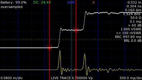
Figure 4: Step TDR vs simulated pulse TDR, x-axis: time/distance, y-axis: reflection coefficient. Top (white) waveform shows step TDR with (from left to right) reflected rise, short 50 Ohm cable inside the instrument, and open reflection at the test port. The vertical level of the signal indicates the impedance of the signal at that point. The lower (yellow) waveform is the associated 1st derivative simulating the appearance of a high-resolution pulse TDR. Impedance information is lost and only gross impedance discontinuities, cable start and open end in this case, are identified. A typical pulse TDR would have 1/10th to 1/100th of the spatial resolution of the yellow trace, however.
Step TDR
Step TDRs use a step-rise excitation signal — a fast rising edge followed by a voltage plateau that lasts at least as long as the sample period. This methodology provides both high spatial resolution and high signal energy for long-range propagation, without the range/resolution trade-off inherent in pulse TDR. In addition, because step TDRs use a continuous excitation source, local impedance variations are clearly delineated as differing reflected voltage levels, and there are no multiple-echo distortion effects like those seen with pulse TDR. The step transition contains useful frequencies ranging from DC to ~0.35/Tr where Tr is the 10-90% system rise time. For a 100 ps rise time TDR, this is approximately 3.5 GHz.
Important Step TDR Parameters
Not all step TDRs are created equal, and paying attention to the system specifications for a given instrument will help you determine the sort of performance you can expect. The most important characteristics of a step TDR are system rise time, cursor resolution, sampling resolution, and sequential sample rate. These largely determine the ability of a step TDR to detect, localize, and characterize cable faults, and are discussed in more detail below.
TDR: System Rise Time
A TDR's system rise time determines the level of detail, and associated frequency content, present in the reflected waveform. The system rise time is determined by the rise times of the instrument's step-rise signal (how quickly the step signal reaches its intended amplitude), and that of the integrated sampling oscilloscope (how fast of a rising or falling edge the sampler can capture). The faster a TDR's system rise time, the sharper its spatial resolution — that is, its ability to separate closely-spaced faults and to detect minor faults. In general, closely spaced faults must be located at least 1/2 of the system rise time apart for them to be separable. This may be important when trying to establish which of two closely spaced connectors is degrading system performance, for example. In addition, cable faults may escape detection or be incorrectly characterized if the spatial resolution is too low. Figure 5 shows two ideal, closely-spaced 1 cm. 75 Ohm partial faults modeled with TDRs of differing system rise times; a slow-rise time TDR system grossly mischaracterizes the faults.
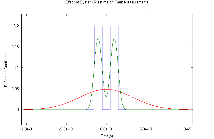
Figure 5: Effect of system rise time on fault measurements. Simulated short-segment (~1 cm. length, ~1 cm. apart) 75 Ohm faults (blue) modeled with TDRs having 90 ps (green), and 800 ps (red) system rise times and 0.8 ps (0.08 mm.) cursor resolution. Horizontal scale is 5 cm/div. The 800 ps rise time system, typical of most portable TDR instruments, grossly mischaracterizes the faults. In addition to having inadequate spatial resolution, most portable TDR instruments would have insufficient timebase/cursor resolution (typically >1 cm.) to adequately depict these faults in the first place.
Because higher frequencies in the test signal are preferentially attenuated by intervening cable, you can expect lower spatial resolution the further out in a cable you test. In addition, intervening interconnects and cable faults will partially attenuate the test signal, exacerbating this effect.
The spatial resolution of a pulse TDR is directly proportional to its pulse width, which is usually at least 1-2 orders of magnitude wider than the rise time of a step TDR like the CT100.
CT100 Series TDRs feature as low as 60 ps rise time (20-80%, CT100HF), for approximately 9 mm. spatial resolution. Typical competing step TDRs have rise times on the order of 600-2000 ps, for spatial resolution of 80-200 mm.
TDR: Timebase Resolution
Timebase resolution, which is often the same as the horizontal cursor resolution displayed on the screen, is the shortest time interval between TDR samples and determines the precision with which cable faults can be localized, the detail with they can be displayed, and the precision with which cable length measurements are made. As with spatial resolution, cable faults may escape detection if the timebase resolution is too coarse — the fault might fall between samples, for instance. Likewise, for applications requiring multiple cables having precisely the same electrical length (i.e. phase-matched cables), the precision of the TDR measurements must exceed the precision of the desired cable matching. Figure 6 shows the effect of shortening a 50 Ohm coaxial cable by approximately 1 mm, measured with the CT100HF.
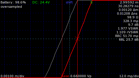
Figure 6: Effect of shaving approximately 1 mm. from the end of a 3 m. coaxial cable; horizontal scale is 1 mm. per major division. Zoomed-in open fault at the end of a 50 Ohm cable saved before (red) and after (white) shaving approximately 1 mm. from the end of the cable. This level of precision is helpful for resolving minor faults, accurately determining cable length for specialized applications (e.g. phase-matched cables), and providing adequate sample density for accurate frequency-domain measurements.
Finally, timebase resolution is critical for TDR frequency-domain measurements using the Fast Fourier Transform (FFT). Sampling resolution less than a few picoseconds is usually necessary for accurate return loss characterization of microwave/RF cables and interconnects.
CT100 Series TDRs feature 760 fs timebase resolution at all cable lengths, equivalent to 0.003 in. (75 μm) in cable with VoP 0.66. This degree of precision is helpful for delineation of short faults, accurate cable phase matching, and frequency-domain measurements to several GHz. Typical competing TDRs have limiting timebase resolution on the order of 0.5-10 in. (1-25 cm.), inadequate for these tasks.
TDR: Sampling Resolution
Sampling resolution refers to the precision with which reflection coefficient measurements are made. CT100 Series TDRs feature up to 60 dB of analog gain coupled to a 16-bit sampler, for precision measurements with wide dynamic range. This allows the operator to detect subtle variations in cable impedance signaling early or minor cable damage, before system performance suffers. Waveforms acquired by the CT100 store all 16 bits of impedance information, much more than can be displayed on the screen. This degree of precision is invaluable for future comparisons — on a subtraction waveform, minor variations in cable or connector performance can be easily detected. Figure 7 shows a waveform acquired at unity gain, displayed at 500 millirho/div, and subsequently zoomed in to show detail at ~1 millirho/div (~0.1 Ohm/div). This level of detail is recorded without operator intervention and can be subsequently displayed on the instrument or with CT Viewer™.
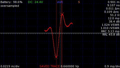
Figure 7: Importance of adequate sampling resolution. A short segment of cable is shown at unity gain in the live waveform (white) with vertical scale set to 500 millirho/div. A scanned waveform acquired directly from the live waveform over this segment is shown (red), subsequently zoomed in vertically to 0.9 millirho/div and showing a 0.5 Ohm variation and 46 dB relative return loss related to an SMA female-female coupler at this location. Because of the subtle detail stored by the CT100 and CT100HF, the operator does not need to be an expert at interpreting TDR to acquire diagnostic information.
TDR: Sequential Sample Rate
Sequential sampling refers to the process by which most step TDRs acquire data — by sequentially sampling point-after-point in successive pulse-echo cycles until a waveform is complete. CT100 Series TDRs feature up to 250 kHz sequential sampling, producing up to 500 full TDR waveforms per second. This allows for the detection of rapid transient faults, speeds smoothing and math transforms, and saves time. Most competing step TDRs are 20-1,000 times slower.
TDR vs. Frequency-Domain Reflectometry (FDR)
FDR is a testing methodology that relies on swept-frequency interrogation of the cable or device-under-test. FDR instruments are valued for quantitatively characterizing the performance of microwave/RF systems in a frequency-specific manner. The inverse Fast Fourier Transform (iFFT) converts frequency-domain information into the time domain for Distance-to-Fault (DTF) estimates. Typical FDR instruments provide bandwidth from 2 MHz or more to an upper limit ranging from 1.6-20 GHz with frequency resolution ranging from 10-100 kHz. FDR and TDR are complementary testing methods that pursue similar measurements using different methods. For general purpose microwave/RF and digital cable and interconnect testing, however, TDR excels in a number of areas, as described below.
TDR vs. FDR: Distance-to-Fault
TDR instruments provide DTF measurements with orders-of-magnitude higher accuracy and precision than those provided by FDR instruments. FDR instruments suffer from an inherent trade-off between horizontal range and resolution, and typically require the operator to select start and stop sweep frequencies to maximize one or the other, regardless of the operating frequency of the system being tested.
Typical FDR testing of a 30 m. cable would provide no better than 5 cm. cursor resolution, nearly 700 times coarser than the CT100. At 1,000 m, this would increase to 1.9 m. To provide the same DTF precision as the CT100 over even 30 m. of cable, an FDR would require a bandwidth of 1300 GHz (the equivalent-time sample rate of the CT100), more than 65 times greater than leading FDR instruments provide. Particularly when testing shorter cables, this lack of horizontal resolution puts FDR at a significant disadvantage relative to TDR.
TDR vs. FDR: Digital Cable Testing
TDR step-rise signals approximate fast digital signals. Characterizing digital cable faults with step TDR is therefore an excellent way to help determine the impact those faults might have on system performance. CT100 Series TDRs' step-rise signals are faster than the fastest digital component families, ensuring that digital communications systems based on these components can be adequately characterized. In addition, TDRs are uniquely suited to testing twisted-pair and non-50 Ohm coaxial cable systems, both of which present significant challenges for FDR instruments.
TDR vs. FDR: Microwave/RF Cable Testing
FDR manufacturers often describe TDR as a "DC" testing methodology that is insensitive to RF. In fact, although TDR waveforms are usually presented in the time domain for ease of interpretation, FDR and TDR are capable of similar frequency-domain measurements. The microwave/RF frequencies carried by a step TDR's rising edge impart nearly all of the diagnostic information an operator uses to detect, localize, and characterize cable faults. CT100 Series TDRs utilize wideband test signals with useful frequency content ranging from DC to more than 8 GHz, and rely on a high-frequency sampler that is exquisitely sensitive to microwave/RF frequencies.
It is important to keep in mind that virtually all cable faults are broadband and preferentially attenuate higher frequencies. Therefore, the best way to find a cable fault quickly is with a broadband test signal, rather than narrowband testing. Testing a system at its operating frequency, which has been claimed as a benefit by FDR manufacturers, would be both insensitive and fail to localize a fault adequately even if it were detected. For this reason, the broadband interrogation provided by a high-resolution step TDR is usually the most effective method to quickly detect and localize microwave/RF cable faults, particularly given TDR's relative ease of use.
If quantitative frequency-specific return loss/VSWR information is desired, well-established methods can be used to provide this information through Fast Fourier Transform (FFT) of time-domain waveforms. This is similar in principle to how FDR instruments provide DTF information through inverse FFT of their frequency-domain measurements.
CT100 Series TDRs feature an FFT math package (currently in beta status), described in more detail elsewhere, that lets the user calculate 1-port S-parameter (S11/S22) values for an estimate of frequency-specific return loss and cable loss. Third-party software solutions that provide this functionality are also available. While these capabilities may not entirely replace the functionality of an FDR instrument, they are acceptable for a number of applications that would also benefit from TDR's highly accurate impedance and DTF measurements. Figure 8 shows a TDR return loss plot from an RG-58 cable using a beta version of the CT100 FFT Math Package, with measurements similar to manufactured cable loss specifications.
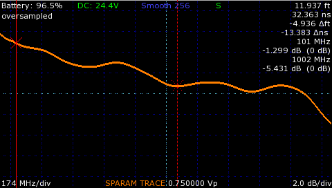
Figure 8: TDR return loss plot of a ~14.3 ft. RG-58 coaxial cable using a beta version of the FFT Math Package. Accounting for connector losses, calculated cable loss at 100 MHz (4.4 dB/100 ft.) and 1 GHz (18 dB/100 ft.) are close to manufactured specification. The FFT Math Package is currently in development.
The misconception that TDR instruments cannot be used for testing microwave/RF systems may be due, at least in part, to the wide availability of low-resolution pulse TDR instruments and their frequent and inappropriate comparison to FDR instruments priced 10-50 times higher. Another potential source of misunderstanding is that while bench-top TDR instruments have been making increasingly accurate microwave/RF frequency-domain measurements for at least 40 years, our CT100 Series TDRs are the first commercially-available portable step TDRs of their kind that provide sufficiently fast system rise time, timebase resolution, and sampling depth to do so.
TDR vs. FDR: Calibration Requirements
FDR, like the Vector Network Analyzer (VNA) technology it is based on, is particularly sensitive to the effects of improper calibration. Calibration typically must be performed in every new testing and environmental situation. Forgetting to perform FDR calibration may result in inaccurate DTF or return loss measurements and associated wasted time and effort.
In contrast, CT100 Series TDRs were designed for a 24-month calibration cycle (12-month calibration cycle is required for NIST traceability), and any timebase variation related to environmental temperature changes over the 0-50°C operating range are internally compensated. Without the need to repeatedly calibrate and recalibrate, cable and interconnect testing is faster and more accurate.
TDR vs. FDR: Transient Faults
FDR is significantly slower than TDR. A CT100 Series TDR acquires a waveform in approximately 2 ms, allowing the instrument to detect rapid transient faults. In contradistinction, because it typically must test hundreds or thousands of frequencies for every measurement, an FDR instrument may require 2-4 s to acquire a waveform. Transient faults could easily be missed or inadequately characterized.
Conclusion
TDR is useful for general testing of modern microwave/RF and digital communications cables and interconnects. The means by which TDR instruments make their measurements and the various system parameters that affect TDR performance are important to keep in mind in order to make the most of a TDR's capabilities.
In particular, Mohr CT100 Series TDRs are uniquely-capable, next-generation TDR instruments designed specifically for troubleshooting and maintenance of coaxial and twisted-pair cables and connectors found in modern microwave/RF and digital systems, and offer significant advantages when compared to competing TDR and FDR instruments.